Getting started#
Contents#
Opening example spectra#
If you want to do this with your own data, make sure it is reduced by following the steps in IRAF
Example ARCES spectra are available online for you to work with. You can
download them via Python like this… this will download temporary copies of
the famous Kepler target KIC 8462852, also known as Boyajian’s Star, and
spectroscopic standard O star BD+28 4211. We also create an
EchelleSpectrum object for each star:
>>> from astropy.utils.data import download_file

>>> target_url = 'https://stsci.box.com/shared/static/mu4fa1fmq1lw8boem12e2umyi99skbdl.fits'
>>> spectroscopic_standard_url = 'https://stsci.box.com/shared/static/18fa008byy2500yrfhuooyxs5d6pwc6e.fits'

>>> target_path = download_file(target_url, show_progress=False)
>>> standard_path = download_file(spectroscopic_standard_url, show_progress=False)

>>> from aesop import EchelleSpectrum

>>> target_spectrum = EchelleSpectrum.from_fits(target_path)
>>> standard_spectrum = EchelleSpectrum.from_fits(standard_path)
You can check basic metadata for an EchelleSpectrum object by printing
it:
>>> print(target_spectrum)
<EchelleSpectrum: 107 orders, 3506.8-10612.4 Angstrom>
The EchelleSpectrum object behaves a bit like a Python list – it
supports indexing, where the index counts the order number, starting with index
zero for the order with the shortest wavelengths. Elements of the
EchelleSpectrum are Spectrum1D objects. Suppose you want to
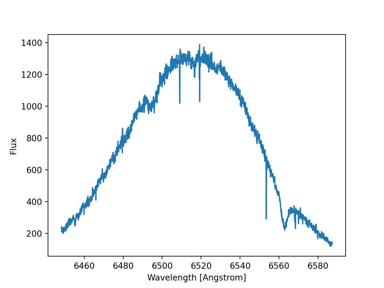
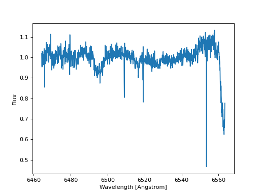
make a quick plot of the 73rd order of the target’s echelle spectrum:
order73 = target_spectrum[73]
order73.plot() # doctest: +SKIP
(Source code, png, hires.png, pdf, svg)
You can see the H-alpha absorption in this O star at 6562 Angstroms.
Normalizing your spectra#
You can continuum-normalize your echelle spectra with two methods:
continuum_normalize_from_standardwill remove the blaze function from each echelle order by fitting polynomials to the continuum of each order of a spectroscopic standard star, and then remove those polynomials from each order of the target starcontinuum_normalize_lstsqwill attempt to remove the blaze function from each echelle order by using a robust least-squares fit to the continuum in each order of the target spectrum – no spectroscopic standard observation is required by this method.
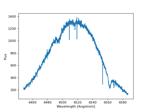
Let’s first use continuum_normalize_from_standard on
our previous example to see order containing the H-alpha line after the blaze
function has been mostly removed:
>>> target_spectrum.continuum_normalize_from_standard(standard_spectrum,
...                                                   polynomial_order=8)
>>> target_spectrum[73].plot()
(Source code, png, hires.png, pdf, svg)

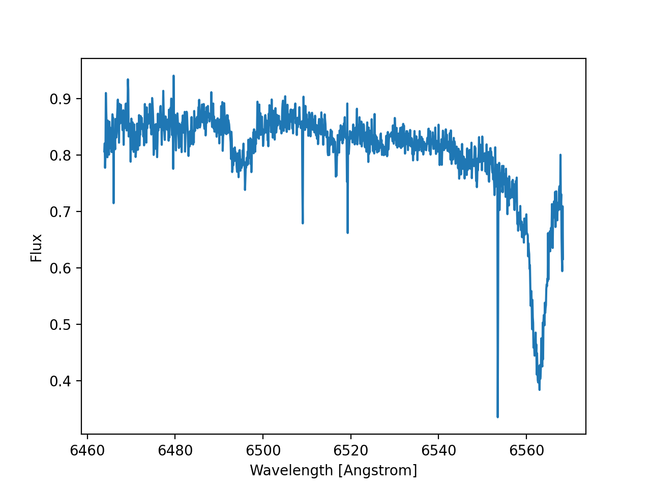
As you can see in this example, the standard star normalization will
approximately flatten the continuum, but not normalize it to unity. We can
now flatten the continuum and normalize it to unity with the other
continuum normalization method,
continuum_normalize_lstsq:
>>> target_spectrum.continuum_normalize_lstsq(polynomial_order=2)
>>> target_spectrum[73].plot()
(Source code, png, hires.png, pdf, svg)
Merge all orders into a 1D spectrum#
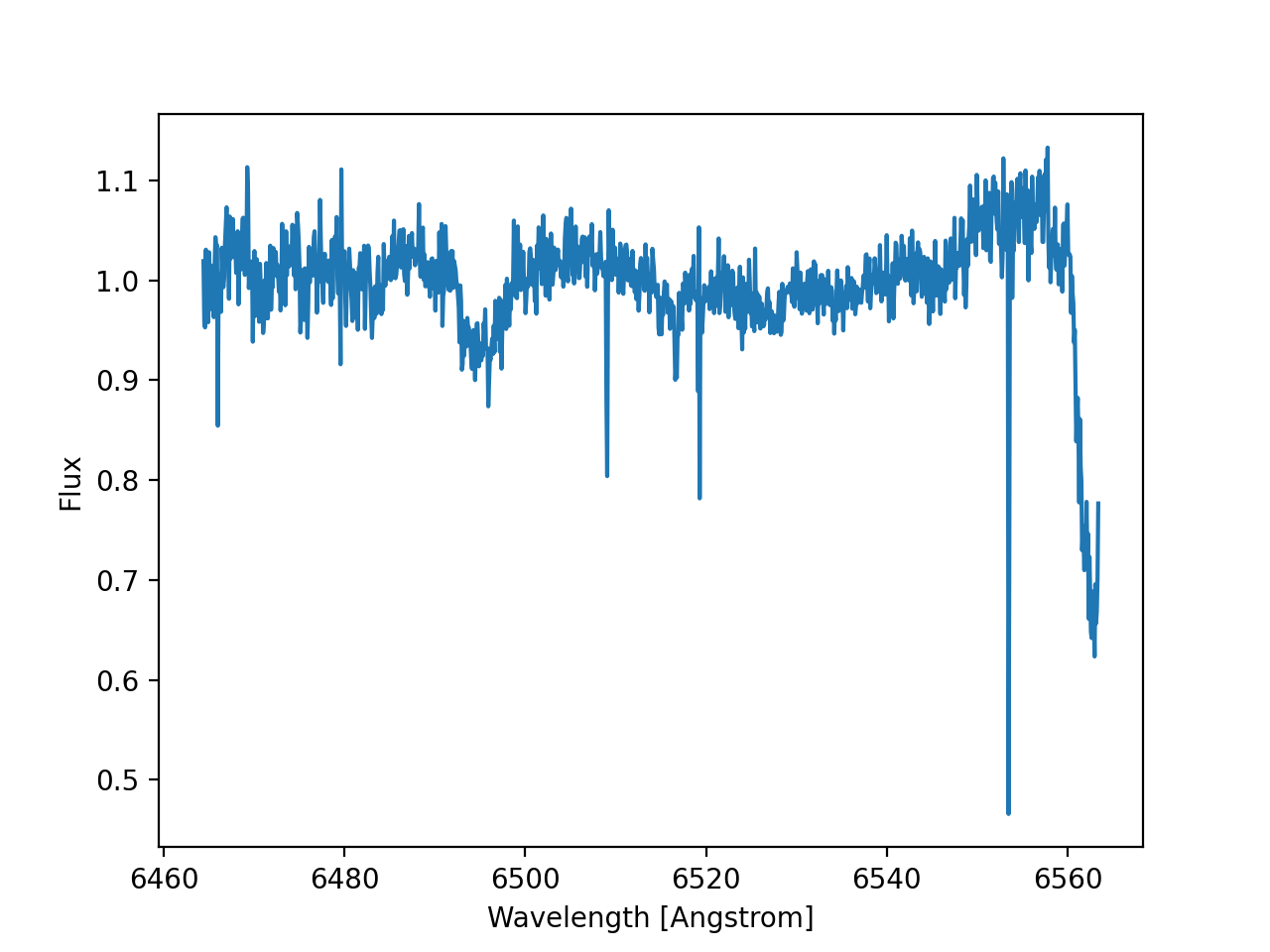
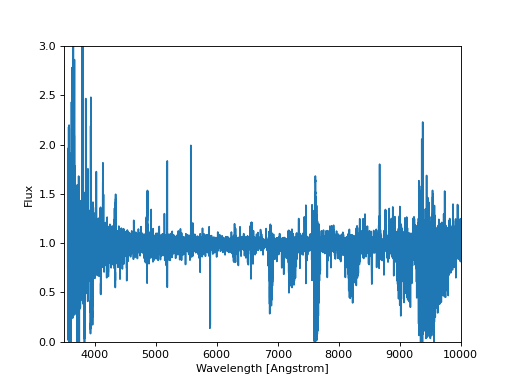
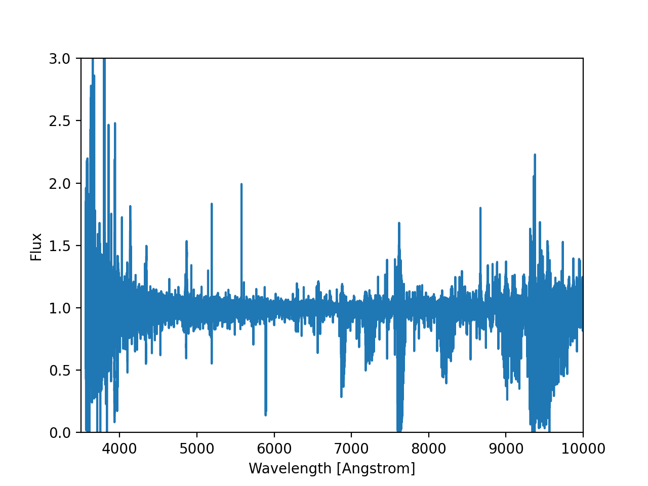
Now that you have a great normalized echelle spectrum, let’s collapse the
echelle spectrum down to one, big 1D spectrum, using
to_Spectrum1D, which will give us a Spectrum1D
object:
>>> spec1d = target_spectrum.to_Spectrum1D()
>>> print(spec1d)
<Spectrum1D: 3562.4-10380.9 Angstrom>

>>> spec1d.plot()
Of course, this plot is going to look a bit bonkers because there is a lot of noise in the extreme red and blue, cosmic rays here and there, and whopping telluric absorption. Here’s what it looks like:
(Source code, png, hires.png, pdf, svg)
